Underground Transmission Line Fault Detection Using MATLAB/Simulink
Underground power cables are the preferred solution for transmission and distribution in urban areas, industrial complexes, and environmentally sensitive zones where overhead lines are restricted or impractical. Compared to aerial conductors, underground cables offer advantages in weather immunity and aesthetics — but when a fault occurs, locating it becomes significantly more challenging. Soil cover means there is no visible flash or broken wire. Accurate, rapid fault detection and location in underground cables is therefore one of the most critical challenges in modern power system engineering.
This article presents a systematic approach to underground cable fault detection and location using MATLAB/Simulink, covering the theoretical basis, simulation modelling methodology, and practical implementation considerations for electrical engineers.
Why Underground Cable Faults Are Different
In overhead transmission lines, faults are predominantly caused by transient phenomena such as lightning, bird strikes, or vegetation contact. Most overhead line faults are temporary and can be cleared by auto-reclosing. Underground cable faults, by contrast, are almost always permanent — typically caused by insulation degradation, dielectric breakdown, mechanical damage during excavation, or moisture ingress. They cannot be cleared by reclosing, and the fault location must be pinpointed before excavation and repair can begin.
Common fault types in underground XLPE (cross-linked polyethylene) and PILC (paper-insulated lead-covered) cables include:
- Single Line to Ground (SLG): most common — one phase conductor contacts the earth sheath
- Line to Line (LL): two phase conductors make contact through insulation breakdown
- Double Line to Ground (DLG): two phases contact the sheath simultaneously
- Three Phase (3P): all conductors short together — rare but most severe
- Open Circuit: conductor breaks internally — voltage present, no current flow
Research shows that approximately 80% of underground cable faults are Single Line to Ground type, driven primarily by insulation aging and moisture ingress at cable joints. MATLAB-based detection systems must prioritise SLG classification accuracy.
— Key Facts
MATLAB/Simulink Modelling Approach
The standard methodology for MATLAB-based underground cable fault detection follows a three-stage process: system modelling, fault simulation, and signal analysis.
Stage 1 — Transmission System Model
An accurate cable model must account for the distributed parameters of the underground cable: resistance, inductance, capacitance, and conductance per unit length. MATLAB/Simulink provides the Distributed Parameter Line block which implements the Bergeron model — the industry-standard travelling wave model for cables.
Key parameters for a typical 11 kV XLPE underground cable model:
| Parameter | Typical Value | Unit |
|---|---|---|
| Positive sequence resistance (R1) | 0.125 | ohm/km |
| Zero sequence resistance (R0) | 0.375 | ohm/km |
| Positive sequence inductance (L1) | 0.3 | mH/km |
| Positive sequence capacitance (C1) | 0.25 | uF/km |
| Surge impedance (Zc) | 34.6 | ohm |
| Propagation velocity | ~175,000 | km/s |
Stage 2 — Fault Simulation
Faults are implemented using the Three-Phase Fault block in Simulink. A Fault Resistance (Rf) parameter represents the actual arc resistance at the fault point — this is critical because high-resistance faults (Rf > 100 ohm) are the most difficult to detect and locate.
A comprehensive fault simulation study should sweep the following variables:
• Fault type: SLG, LL, DLG, 3P (4 configurations)
• Fault location: every 10% of cable length from 10% to 90% (9 positions)
• Fault resistance: 0.1 ohm, 1 ohm, 10 ohm, 100 ohm (4 levels)
• Fault inception angle: 0°, 45°, 90°, 135° (4 angles)
This gives a simulation matrix of 576 cases — comprehensive enough to train and validate a fault classifier.
Stage 3 — Signal Analysis Methods
Raw current and voltage waveforms from the fault simulation are processed using signal analysis techniques to extract features for fault detection and location.
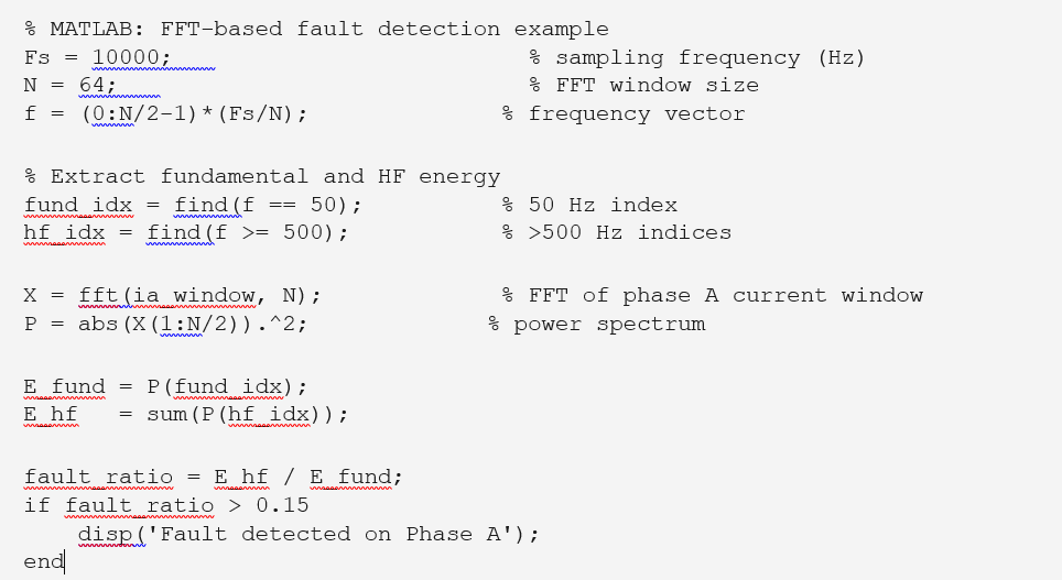
Fast Fourier Transform (FFT) Based Detection
The FFT decomposes the fault current signal into its frequency components. During a fault, the current waveform contains significant high-frequency content not present in the normal pre-fault signal. The FFT-based detection algorithm:
- Samples the three-phase current at both ends of the cable at 10 kHz
- Applies a 64-point FFT to each 6.4 ms window of data
- Computes the ratio of high-frequency energy (500 Hz to 5 kHz) to fundamental frequency energy
- Compares this ratio against a threshold — fault is declared if ratio exceeds 0.15
- Classifies fault type based on the combination of phases showing elevated HF content
hi
Pradip Subedi
Electrical Consultancy
Specialized in electrical installation, solar systems and industrial maintenance. Based in Kathmandu, Nepal with 5+ years of hands-on field experience.
Related Articles
More articles you might find useful.